 NexGPU-算力租赁,GPU服务器,GPU云算力,AI服务器租用-新闻博客
In mid-2026, NVIDIA Blackwell Ultra (B300) launched. Facing B200's rental price, can paying about 1.75x the hourly rate be justified by topology simplification? This article provides answers using a cost-per-token framework.
1. After B300's Launch, How Has the Price Tier of High-End Cards Been Reshaped?
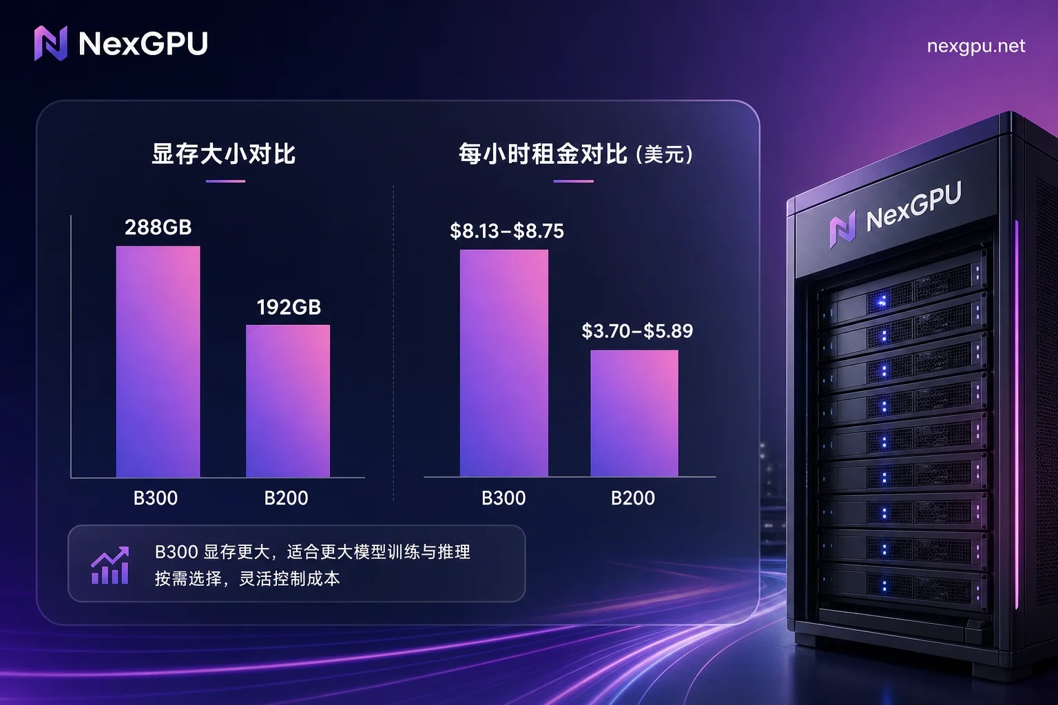
B300 (Blackwell Ultra) has public specs of 288GB HBM3e memory (public specs from 2026) and 15 PFLOPS dense FP4 compute (public specs from 2026). Memory capacity is 50% higher than B200's 192GB, and dense compute performance is 1.5x higher. In mid-2026 cloud compute platform public data, B300's on-demand rental median price is $8.13-$8.75/GPU-hour (public quotes from cloud platforms, June-July 2026), while B200's per-card rental ranges from $3.70-$5.89/hour (public quotes from cloud platforms, June-July 2026). By median price, B300's hourly rate is about 1.7-1.8x B200's, but memory is only 50% more. This is not linear; if B300 cannot deliver proportional throughput gains or reduction in node count, it may only be a paper performance champion. Previous cost-performance conclusions for B200 and H100 need to be recalculated under real workloads. Note: all prices and specs in this article come from publicly available 2026 data; no unverified benchmark data is cited.
2. 288GB vs 192GB: What Kind of Problems Does the 50% Memory Increase Actually Solve?
The 96GB memory increase seems like just a capacity change, but the benefiting scenarios are step-like. First, large-parameter model weight residency: when model weights plus KV Cache exceed 192GB, B200 cannot fit on a single card, usually requiring tensor parallelism across multiple cards within a node; only when the whole node's memory is insufficient do you need cross-node. The real cost leap comes from "cross-node", not "cross-card". B300 might fit in a single node, saving communication overhead. Second, long-context scenarios: doubling context length increases KV Cache almost linearly, e.g., a 100B model, expanding context from 32K to 128K, KV Cache may increase by tens of GB, which is where 288GB memory shines.
But note, memory gains do not apply to all models. If your model's weights plus KV Cache are far below 192GB, or concurrency is low, the 50% memory increase is just redundancy and cannot translate into cost advantage. So, 288GB's value lies in whether it crosses the threshold of "model fitting on a single card or node". So, what size models can 288GB accommodate? Under FP8, models with weights up to about 230GB have a chance for single-card residency, but it still depends on KV Cache and framework overhead; use the formula in Section 3 to estimate.
3. Converting Memory Capacity to Node Count: What Scale of Models Move from Cross-Node to Single-Node?
Below is an estimation method example; replace parameters with your own workload.
Required memory ≈ (Parameters in B) × (Bytes per parameter) + KV Cache size + Framework and activation overhead (usually leave 20% headroom)
For example, a 700B parameter model using FP8 (1 byte per parameter), with estimated KV Cache of 100GB (assumed value, not measured), total requirement = 700GB + 100GB = 800GB, plus 20% headroom = 800GB × 1.2 = 960GB. If each node has 4 cards (example setting), B200 single card 192GB, required cards = 960 ÷ 192 = 5 cards, with 4 cards per node (example setting) requiring 2 nodes; B300 single card 288GB, required cards = ceil(960/288) = 4 cards, single node suffices. Node count drops from 2 to 1, saving not only cross-node communication latency but also network bandwidth rental costs.
But if parameters drop to 100B, weights about 100GB (FP8), whether KV Cache exceeds 192GB depends on context length and concurrency; plug in your own values using the above formula. If not, B200 single card suffices, and B300's memory increase does not change node count, making the extra hourly rate pure premium.
4. 15 PFLOPS Dense FP4 and 1.5x Compute Increase: How Much Remains in Actual Throughput?
Paper compute increase is an upper bound, not expected gain. Actual throughput is limited by three factors: memory bandwidth bottlenecks, batching organization, and bandwidth characteristics in the decode phase. In generative inference, repeated reads of KV Cache often leave the GPU memory-bandwidth-bound, not compute-bound. B300's 15 PFLOPS dense FP4 is peak, but if the model is not quantized to FP4 (which may cause accuracy loss), or operator libraries are not fully optimized, actual throughput may be far below 1.5x.
The data package did not provide measured B300 throughput, so here we only provide a judgment framework, key points:
- Prefill vs. Decode: Prefill is usually compute-bound; decode is usually bandwidth-bound. Peak compute gains are more likely reflected in prefill; if your workload is dominated by long decode, compute gains may be greatly reduced.
- FP4 Quantization Accuracy Regression: If adopting FP4 quantization, compare accuracy drop on validation set before and after quantization to see if acceptable; if not, cannot utilize FP4 peak.
- Batch and Concurrency Impact: Peak utilization often requires high batch size; if your concurrency is sparse, actual throughput may be far below peak.
These are judgment frameworks, not measurements; validate with your own workload.
5. Unit Price ≠ Cost: A Reusable Formula for Cost per Million Tokens
Core formula:
Cost per million tokens = (Number of cards × Hourly rate) ÷ (Measured throughput × 3600) × 10⁶
Where measured throughput is in tokens/s. Additionally, three corrections:
- Utilization: actual workloads don't always run at full capacity, typically discounted to 70%-85%;
- Node count amplification factor: if cross-node, consider communication overhead causing throughput loss;
- Long-tail concurrency redundancy: reserve 10%-30% compute for peak.
Use public rental price ranges to demonstrate reverse solving (example algorithm, assumed values not measured; replace with your measurements): Assume a model on B200 has measured throughput 2000 tokens/s, single card (no cross-node), median price $4.8/hour. B300 median price $8.4/hour. To match unit cost without changing node count (assuming both single card), required B300 throughput: Throughput_B300 = 2000 × (8.4/4.8) ≈ 3500 tokens/s, about 1.75x B200. This threshold is higher than B300's paper compute increase of 1.5x, so in scenarios where node count unchanged, B300 may not match unit cost via throughput alone. If B300 reduces node count from 2 to 1 due to ample memory, while B200 needs 2 nodes, then B200 cost doubles, making B300 perhaps worthwhile.
6. Why Didn't B300's Launch Immediately Make B200 and H100 Lose Value?
B300 is positioned for large models and long contexts, not a universal replacement. For medium-scale inference where memory is not a bottleneck, B200 at $3.70-$5.89/hour (public quotes from cloud platforms, June-July 2026) still has clear cost-effectiveness. B300's launch does not automatically lower old card prices—data package provides no evidence of price changes, so speculation is unwarranted. The price tiers are layered: consumer cards at low end, B200 at mid, B300 at high, each in its place.
Whether to stick with H100 or switch to B200 can be judged from three dimensions:
- Ecosystem and operator stability: H100's CUDA ecosystem is mature; if your production stack deeply relies on its operator library, migration costs may exceed compute gains.
- Depreciation of existing assets: If you already own H100 assets, consider depreciation costs first, not just rental prices.
- Memory bottleneck exposure: If your current model on H100 does not show memory overflow or cross-node needs, urgency to switch to B200 is low; if memory is near limit, B200's 192GB becomes attractive.
The above is positioning and methodology discussion, not regarding specific specs and prices.
7. The Lower Bound: Demands That 32GB Consumer Cards Can Meet Should Not Be Hijacked by High-End Card Narratives
In July 2026, cloud monitoring data showed RTX 5090's 32GB GDDR7 memory rental at $0.47-$0.56/hour (multi-platform monitoring data late July 2026), bandwidth 1.79 TB/s, 30%-70% higher throughput than RTX 4090. Meanwhile, 16GB RTX 5080 (about $0.22/hour, multi-platform monitoring data late July 2026) easily overflows VRAM when running models larger than 8B or not heavily quantized. 32GB memory can run 32B models and concurrent KV Cache without overflow. This means if your model is below 30B and you don't pursue extremely long contexts, consumer cards are sufficient; no need to jump to the $8 tier.
8. Four-Tier Decision Table: When to Stay on H100, When to Upgrade to B200, When B300 Is Necessary, and When Consumer Cards Are Enough
| Trigger Condition | Recommended Tier | Judgment Basis | Verification Method (Requires Measurement) |
|---|---|---|---|
| Model <32B, medium context and concurrency, memory needs don't hit single-card limit | Consumer card (e.g., RTX 5090) | 32GB memory without overflow, hourly rate <$1 | Memory peak, throughput |
| Existing H100 assets, strong ecosystem dependence, and model memory needs don't hit single-card limit | H100 (positional description) | This article does not cite its specific memory and price data; use your measurements with Section 5 formula | Throughput, memory peak |
| Model 32B-100B, medium context, single-card memory sufficient | B200 or H100 | Single-card memory sufficient, no cross-node needed; if cross-node, refer to B300 tier | Memory peak, cross-node status, throughput |
| Model >100B, long context, or cross-node required | B300 | 288GB fits in single node, saving communication cost; if cross-node, consider B300 | Node count, throughput, P99 latency |
Actual selection should combine Section 5 formula for cost and verify with measurements.
9. Conducting a Cross-Generation Same-Workload Comparison Test with On-Demand Resources: Steps and Checklist
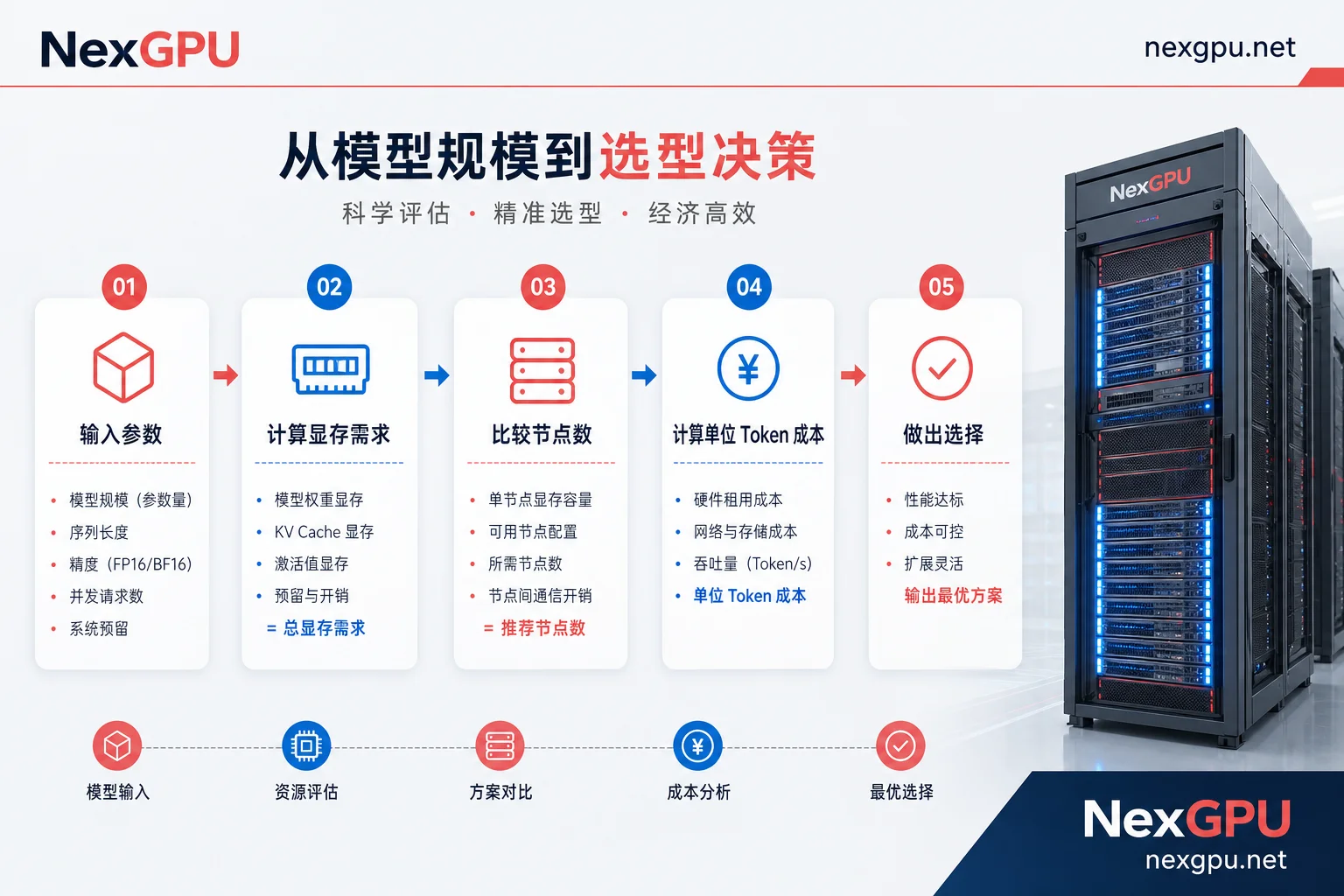
To get your own cost per million tokens, follow these steps for A/B testing:
- Fix model, context length distribution, and concurrency curve.
- On a platform that supports multiple GPU types, pay-as-you-go, and instant availability (e.g., NexGPU), run the same workload on short-cycle on-demand instances, then release after testing.
- Record measured throughput, P99 latency, memory peak, and utilization.
- Plug into Section 5 formula to compute the unit token cost for each option.
First use the Section 5 formula with your actual workload to calculate cost per token, then run a cross-tier comparison test with on-demand resources, and finally decide on the purchase tier. Any paper comparison is inferior to measured data—your model, your workload, are the ultimate decision basis.




Comments(0)